10 Minutes to GFQL

Welcome to GFQL (GraphFrame Query Language), the first dataframe-native graph query language. GFQL brings graph queries to data science workflows without an external graph database. It works with the PyData, Apache Arrow, and GPU ecosystems, so large graphs run in-process on CPU or GPU.

In this guide, we’ll explore the basics of GFQL in just 10 minutes. You’ll learn how to:

• Query and filter nodes and edges.

• Chain multiple hops and apply predicates.

• Use automatic GPU acceleration.

• Integrate GFQL into your existing Python workflows.

• Run GFQL and Python on remote GPUs and remote data.

Introduction to GFQL

GFQL is an in-process graph query language for the compute tier. Graph databases couple storage and compute; GFQL queries the dataframes you already have, in memory, on CPU or GPU.

Key Benefits:

• Dataframe-Native: Works directly with Pandas, Polars, cuDF, and other dataframe libraries.

• High Performance: Optimized for both CPU and GPU execution.

• Ease of Use: No need for external databases or new infrastructure.

• Interoperability: Integrates with the Python data science ecosystem, including PyGraphistry for visualization.

Sample Dataset

Throughout this guide, we’ll work with a graph representing people, companies, and transactions with risk indicators:

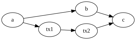
Sample graph rendered with plot_static().

import pandas as pd
import graphistry

nodes_df = pd.DataFrame({
    'id': ['a', 'b', 'c', 'tx1', 'tx2'],
    'type': ['person', 'person', 'company', 'transaction', 'transaction'],
    'risk1': [False, False, False, True, False],
    'risk2': [False, False, False, False, True],
})
edges_df = pd.DataFrame({
    'src': ['a', 'b', 'a', 'tx1', 'tx2'],
    'dst': ['b', 'c', 'tx1', 'tx2', 'c'],
    'e_type': ['knows', 'works_at', 'sent', 'transfer', 'received'],
    'interesting': [True, True, False, False, False],
})

g = graphistry.edges(edges_df, 'src', 'dst').nodes(nodes_df, 'id')

Setting Up GFQL

GFQL is part of the open-source graphistry library. Install it using pip:

pip install graphistry

Ensure you have pandas or cudf installed, depending on whether you want to run on CPU or GPU.

Two Syntax Styles

GFQL supports two syntax styles through the same g.gfql(...) entrypoint:

Cypher strings — familiar if you know SQL or Cypher:

# Filter nodes — returns a DataFrame
nodes_df = g.gfql("MATCH (n {type: 'person'}) RETURN n")._nodes

# Extract a subgraph — returns a graph with ._nodes and ._edges
g2 = g.gfql("GRAPH { MATCH (a)-[e]->(b) WHERE e.interesting = true }")

Native chain syntax — composable Python objects:

from graphistry import n, e_forward

# Same node filter, chain form
nodes_df = g.gfql([ n({"type": "person"}) ])._nodes

# Same subgraph extraction, chain form
g2 = g.gfql([ e_forward({"interesting": True}) ])

Both styles run on the same vectorized engine, with the same CPU/GPU acceleration. Use whichever you prefer — or mix them.

Examples

1. Find Nodes of a Certain Type

# Cypher style — returns a DataFrame of matching nodes
nodes_df = g.gfql("MATCH (n {type: 'person'}) RETURN n")._nodes

# Equivalent chain style
from graphistry import n
nodes_df = g.gfql([ n({"type": "person"}) ])._nodes
# nodes_df: DataFrame with 'a' and 'b' (the person nodes)

2. Find 2-Hop Edge Sequences with an Attribute

Traverse multiple hops and filter edges based on attributes.

# Cypher style — GRAPH { } returns a subgraph with ._nodes and ._edges
g2 = g.gfql("GRAPH { MATCH (a)-[e]->(b) WHERE e.interesting = true }")

# Equivalent chain style
from graphistry import e_forward
g2 = g.gfql([ e_forward({"interesting": True}, hops=2) ])
# g2._edges: edges a->b->c (both marked interesting)
g2.plot()

Explanation:

• e_forward({"interesting": True}, hops=2) traverses forward edges with interesting == True for 2 hops.

• g_2_hops.plot() visualizes the resulting subgraph.

3. Find Nodes 1-2 Hops Away and Label Each Hop

Label hops in your traversal to analyze specific relationships.

Example: Find nodes up to 2 hops away from node “a” and label each hop

from graphistry import n, e_undirected

g_2_hops = g.gfql([
    n({g._node: "a"}),
    e_undirected(name="hop1"),
    e_undirected(name="hop2")
])
first_hop_edges = g_2_hops._edges[ g_2_hops._edges.hop1 == True ]
# first_hop_edges: edges directly connected to 'a' (hop1=True)

The Cypher form returns the same subgraph. Cypher has no per-hop label, so use the chain form when you need the hop1 / hop2 columns:

g_2_hops_cypher = g.gfql("GRAPH { MATCH (a {id: 'a'})-[hop1]-(b)-[hop2]-(c) }")
assert set(g_2_hops_cypher._nodes['id']) == set(g_2_hops._nodes['id'])

Explanation:

• n({g._node: "a"}) starts the traversal from node "a" where g._node is the identifying column name.

• e_undirected(name="hop1") traverses undirected edges and labels them as hop1.

• e_undirected(name="hop2") continues traversal and labels edges as hop2.

• The labels allow you to filter and analyze edges from specific hops.

4. Query for Transaction Nodes Between Risky Nodes

Chain multiple traversals to find patterns between nodes.

Example: Find risk2 transactions reachable from risk1 nodes

from graphistry import n, e_forward

g_risky = g.gfql([
    n({"risk1": True}),
    e_forward(to_fixed_point=True),
    n({"type": "transaction", "risk2": True}, name="hit")
])
hits = g_risky._nodes[ g_risky._nodes["hit"] == True ]
assert sorted(hits['id']) == ['tx2']
# hits: transaction nodes flagged risk2 that a risk1 node reaches (tx1 -> tx2)

The Cypher form uses a variable-length path for to_fixed_point:

hits_df = g.gfql(
    "MATCH (r {risk1: true})-[*1..]->(t {type: 'transaction', risk2: true}) "
    "RETURN t.id AS id"
)._nodes
assert sorted(hits_df['id']) == ['tx2']

Explanation:

• Starts from nodes with risk1 == True (tx1).

• Follows forward edges to a fixed point (every node reachable from the start set).

• Keeps transaction nodes with risk2 == True and labels them hit (tx2).

5. Filter by Multiple Node Types Using is_in

Use the is_in predicate to filter nodes or edges by multiple values.

Example: Filter nodes and edges by multiple types

from graphistry import n, e_forward, is_in

g_filtered = g.gfql([
    n({"type": is_in(["person", "company"])}),
    e_forward({"e_type": is_in(["sent", "transfer"])}, to_fixed_point=True),
    n({"type": is_in(["transaction", "account"])}, name="hit")
])
hits = g_filtered._nodes[ g_filtered._nodes["hit"] == True ]
assert sorted(hits['id']) == ['tx1', 'tx2']
# hits: transaction/account nodes reached over sent/transfer edges (a -> tx1 -> tx2)

In Cypher, is_in is IN. This single-hop form returns the first transaction; variable-length paths with IN filters on several aliases are not yet supported (#2019):

hits_df = g.gfql(
    "MATCH (a)-[e]->(t {type: 'transaction'}) "
    "WHERE a.type IN ['person', 'company'] AND e.e_type IN ['sent', 'transfer'] "
    "RETURN t.id AS id"
)._nodes
assert sorted(hits_df['id']) == ['tx1']

Explanation:

• Filters start nodes of type "person" or "company".

• Follows forward edges of type "sent" or "transfer" to a fixed point.

• Keeps nodes of type "transaction" or "account" and labels them hit.

Using GPU Acceleration

GFQL is optimized for GPU acceleration using cudf and rapids. When using GPU dataframes, GFQL automatically executes queries on the GPU for massive speedups.

6. Automatic GPU Acceleration

Example: Run GFQL queries with GPU dataframes

import cudf
import graphistry

# Load data into GPU dataframes
e_gdf = cudf.read_parquet('edges.parquet')
n_gdf = cudf.read_parquet('nodes.parquet')

# Create a graph with GPU dataframes
g_gpu = graphistry.edges(e_gdf, 'src', 'dst').nodes(n_gdf, 'id')

# Run GFQL query (executes on GPU); Cypher strings work the same way
g_result = g_gpu.gfql([ ... ])
g_result = g_gpu.gfql("MATCH (n {type: 'person'}) RETURN n")

Explanation:

• cudf.read_parquet() loads data directly into GPU memory.

• GFQL detects cudf dataframes and runs the query on the GPU.

• Achieves significant performance improvements on large datasets.

7. Selecting an Engine (CPU and GPU)

You can explicitly set the execution engine. The same query returns identical results on every engine — see Choosing an Engine.

Example: CPU columnar speedup (no GPU)

people = g.gfql("MATCH (n {type: 'person'}) RETURN n", engine='polars')._nodes
assert len(people) == 2   # same answer as the pandas engine

Example: Force GFQL to use a GPU engine

g_result = g_gpu.gfql([ ... ], engine='cudf')        # NVIDIA GPU, eager
g_result = g_gpu.gfql([ ... ], engine='polars-gpu')  # NVIDIA GPU, fused plan

Explanation:

• engine='polars' runs the columnar CPU engine — the biggest win without a GPU.

• engine='cudf' / 'polars-gpu' force GPU-accelerated execution.

• Useful when you want to ensure the query runs on a specific engine.

Integration with PyData Ecosystem

GFQL works with the PyData ecosystem, so you can combine it with libraries like pandas, networkx, igraph, and PyTorch.

8. Combining GFQL with Graph Algorithms

Example: Compute PageRank on the resulting graph

# Assuming g_result is the result from a GFQL query

# Compute PageRank using cuGraph (GPU)
g_enriched = g_result.compute_cugraph('pagerank')

# View top nodes by PageRank
top_nodes = g_enriched._nodes.sort_values('pagerank', ascending=False).head(5)
# top_nodes[['id', 'pagerank']]: DataFrame with highest PageRank nodes

Explanation:

• compute_cugraph('pagerank') computes the PageRank of nodes using GPU acceleration.

• The enriched graph now contains a pagerank column in the nodes dataframe.

9. Visualizing the Graph

Use PyGraphistry’s visualization capabilities to explore your graph.

Example: Visualize high PageRank nodes

from graphistry import n, e

# Filter nodes with high PageRank
g_high_pagerank = g_enriched.gfql([
    n(query='pagerank > 0.1'),
    e(),
    n(query='pagerank > 0.1')
])

# Plot the subgraph
g_high_pagerank.plot()

Explanation:

• Filters nodes where pagerank > 0.1.

• Visualizes the subgraph consisting of high PageRank nodes.

10. Sequencing Programs with Let

GFQL’s Let bindings enable you to sequence complex graph programs as directed acyclic graphs (DAGs). This allows you to build sophisticated analysis pipelines with named operations that reference each other:

Example: Multi-stage fraud analysis

from graphistry import let, ref, call, n, e_forward, e, gt

result = g.gfql(let({
    # Stage 1: Find suspicious accounts
    'suspicious_accounts': n({'risk_score': gt(80), 'created_recent': True}),

    # Stage 2: Trace money flows from suspicious accounts
    'money_flows': [
        n({'risk_score': gt(80), 'created_recent': True}),
        e_forward({'type': 'transfer', 'amount': gt(10000)}, hops=3),
        n()
    ],

    # Stage 3: Compute PageRank to find central nodes
    'ranked': ref('money_flows', [
        call('compute_cugraph', {'alg': 'pagerank'})
    ]),

    # Stage 4: Identify high-risk clusters
    'high_risk_clusters': ref('ranked', [
        n({'pagerank': gt(0.01)}),
        e(),
        n(),
        call('compute_cugraph', {'alg': 'louvain'})
    ])
}))

# Access results from each stage
suspicious = result._nodes[result._nodes['suspicious_accounts']]
clusters = result._nodes[result._nodes['high_risk_clusters']]
# suspicious: nodes flagged in stage 1
# clusters['community']: community assignments from stage 4

Key benefits of Let bindings:

• Declarative DAG: Express complex multi-stage analysis as a clear computation graph

• Efficient execution: All stages execute in a single optimized pass

• Named results: Access intermediate results by name for detailed analysis

• Composability: Build complex patterns from simpler named operations

11. Run remotely

You may want to run GFQL remotely because the data is remote or a GPU is available remotely:

Example: Run GFQL remotely

from graphistry import n, e

g2 = g1.gfql_remote([n(), e(), n()])

Example: Run GFQL remotely, and decouple the upload step

from graphistry import n, e

g2 = g1.upload()
assert g2._dataset_id is not None, "Uploading sets ``dataset_id`` for subsequent calls"
g3 = g2.gfql_remote([n(), e(), n()])

Additional parameters enable controlling options such as the execution engine and what is returned

Example: Bind to existing remote data and fetch it

import graphistry
from graphistry import n

g2 = graphistry.bind(dataset_id='my-dataset-id')

nodes_df = g2.gfql_remote([n()])._nodes
edges_df = g2.gfql_remote([e()])._edges

Example: Run Python on remote GPUs over remote data

def compute_shape(g):
    g2 = g.materialize_nodes()
    return {
        'nodes': g2._nodes.shape,
        'edges': g2._edges.shape
    }

g = graphistry.bind(dataset_id='my-dataset-id')
shape_info = g.python_remote_json(compute_shape)
# shape_info: {'nodes': (1000, 5), 'edges': (5000, 3)}

Example: Run Python on remote GPUs and return a graph

def compute_shape(g):
    g2 = g.materialize_nodes()
    return g2

g = graphistry.bind(dataset_id='my-dataset-id')
g2 = g.python_remote_g(compute_shape)
# g2._nodes: DataFrame returned from remote execution

Conclusion and Next Steps

Congratulations! You’ve covered the basics of GFQL in just 10 minutes. You’ve learned how to:

• Query and filter nodes and edges using GFQL.

• Chain multiple hops and apply advanced predicates.

• Use GPU acceleration for large graphs.

• Integrate GFQL with graph algorithms and visualization tools.

Next Steps:

• Try GFQL on Your Data: Apply what you’ve learned to your datasets and see the benefits firsthand.

• Translate Between SQL, Pandas, Cypher, and GFQL

• GFQL Quick Reference

• 10 Minutes to PyGraphistry: Utilize PyGraphistry for advanced visualization and analysis.

• Join the Community: Connect with other users and developers in the GFQL community Slack channel.

GFQL runs graph analysis at scale without a database to manage. It fits the Python ecosystem and moves to a GPU with one keyword.

Happy graph querying!